Download the SPARKTA 2 2026 (Next-Gen Engineering Simulation) Software Download from this link…
![]()
Overview of the Software
Table of Contents
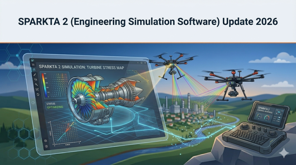
SPARKTA 2 is a high-performance engineering simulation platform designed for finite element analysis (FEA), computational fluid dynamics (CFD), and thermal-structural coupling. Released as the 2026 major update, SPARKTA 2 introduces a unified solver environment that bridges the gap between mechanical, aerospace, and civil engineering workflows.
Unlike traditional simulation tools, SPARKTA 2 focuses on real-time iterative analysis, allowing engineers to modify boundary conditions and see updated results without full recomputation. The 2026 update prioritizes cloud-native hybrid processing, GPU-accelerated solvers, and an overhauled meshless algorithm for complex geometries. This version is primarily targeted at mid-to-large engineering firms, research institutions, and advanced product design teams.
As a multiphysics simulation software, SPARKTA 2 competes directly with established tools while offering faster convergence rates for nonlinear problems. Whether you are performing structural integrity checks, vibration analysis, or heat transfer simulations, SPARKTA 2 aims to reduce solve times by up to 40% compared to its previous version.
Key Features
SPARKTA 2 includes the following core capabilities:
-
Meshless Domain Decomposition – Eliminates traditional meshing bottlenecks for complex assemblies.
-
Adaptive Solver Engine – Automatically switches between direct and iterative solvers based on matrix conditioning.
-
Real-Time Parameter Sweep – Visualize stress, strain, and temperature variations across 50+ input parameters simultaneously.
-
CAD-Native Integration – Direct import of STEP, IGES, Parasolid, and native SolidWorks/Autodesk Inventor files.
-
Multi-GPU Support – Scales linearly across NVIDIA RTX and AMD Instinct accelerators.
-
Python API for Automation – Script parametric studies, optimization loops, and result extraction.
-
Built-in Material Library 2026 – Includes 1,200+ materials with temperature-dependent properties and composite layup definitions.
-
Cloud Burst Mode – Offloads transient or nonlinear runs to AWS or Azure without leaving the desktop UI.
These features position SPARKTA 2 as a viable alternative for teams requiring both accuracy and iteration speed.
What’s New in SPARKTA 2 Update 2026
The 2026 update is not a minor patch but a substantial version upgrade. Key improvements include:
-
New Solver: Dynamic Explicit with HF Integration – Handles drop tests, impact, and crashworthiness simulations 3x faster.
-
AI-Assisted Boundary Condition Detection – Automatically identifies fixed faces, symmetry planes, and load-bearing surfaces from CAD geometry.
-
Fatigue Life Predictor Module – SN-curve and strain-life methods with rainflow cycle counting integrated into post-processing.
-
Live Dashboard for Residual Analysis – Monitor convergence history, energy norms, and force residuals during solution.
-
Improved HPC Scaling – Now supports up to 256 cores on-premise and 1,024 cores in cloud burst.
-
Native Linux Workstation Build – Full command-line batch processing for CI/CD simulation pipelines.
-
Expanded Results Export – VTK, Ensight, and HDF5 formats alongside native SPARKTA binary.
This update substantially improves usability for advanced nonlinear transient problems and fatigue analysis.
System Requirements
To run SPARKTA 2 Update 2026 efficiently, ensure your hardware meets the following specifications:
Minimum Requirements (Small assemblies, <50k DOF)
-
OS: Windows 10/11 Pro (64-bit) or Ubuntu 22.04/24.04 LTS
-
CPU: 6-core Intel Core i7 or AMD Ryzen 5 (3.2 GHz+)
-
RAM: 16 GB DDR4
-
GPU: Integrated or basic discrete (no GPU acceleration required)
-
Storage: 25 GB SSD
-
Display: 1920×1080, DirectX 11 compatible
Recommended Requirements (Standard use, up to 500k DOF)
-
OS: Windows 11 Pro for Workstations or Ubuntu 24.04 LTS
-
CPU: 16-core Intel Xeon W or AMD Threadripper
-
RAM: 64 GB DDR5 ECC
-
GPU: NVIDIA RTX 4070 / A2000 (12 GB VRAM) or AMD Radeon Pro W7700
-
Storage: 1 TB NVMe SSD
-
Display: 2560×1440 dual monitors
High-Performance (Multiphysics & transient, >2M DOF)
-
OS: Ubuntu 24.04 or Windows Server 2022
-
CPU: Dual 32-core AMD EPYC (Genoa) or Intel Xeon Scalable
-
RAM: 256 GB to 1 TB DDR5 ECC
-
GPU: 2x NVIDIA RTX 6000 Ada or 4x RTX 4090 (for explicit solvers)
-
Storage: 4 TB NVMe RAID 0
-
Network: 10 GbE for cluster jobs
Installation Guide
Follow this step-by-step guide for a clean installation of SPARKTA 2 Update 2026.
Pre-Installation Checklist
-
Verify system compatibility (see section above).
-
Uninstall previous versions of SPARKTA or conflicting simulation software.
-
Disable real-time antivirus temporarily (add exclusion paths afterward).
-
Ensure Windows: Install Visual C++ Redistributables (2015-2022).
Linux: Installlibgl1,libstdc++6, andopenmpi-bin.
Installation Steps (Windows)
-
Download the official installer from your SPARKTA customer portal.
-
Right-click
SPARKTA2_2026_setup.exe→ Run as Administrator. -
Choose Custom Installation → Select components:
-
Core Solver (required)
-
Python API + Examples
-
Material Database 2026
-
Cloud Connector Module
-
-
Set installation path (avoid spaces, e.g.,
C:\SPARKTA2_2026). -
License activation: Enter your node-locked or floating license server address.
-
Complete installation and restart your workstation.
Installation Steps (Ubuntu Linux)
chmod +x sparkta2_2026_linux.bin
sudo ./sparkta2_2026_linux.bin --prefix /opt/sparkta2
export PATH=/opt/sparkta2/bin:$PATH
sparkta2 license activate --server 192.168.1.100:27000
How to Use the Software
This section covers the core workflow for a typical structural-thermal simulation.
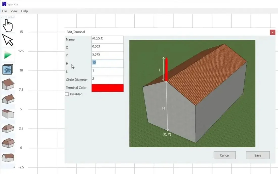
Step 1 – Geometry Import
-
Click File → Import CAD.
-
Select your native CAD file (STEP recommended for best topology).
-
Use Repair Tools → stitch surfaces, remove duplicate faces.
Step 2 – Material Assignment
-
Open Material Library.
-
Search by name or property (e.g., “AISI 4340 steel at 500°C”).
-
Drag material onto part or assembly.
Step 3 – Boundary Conditions and Loads
-
Fixed support: Right-click model tree → Fixed Displacement.
-
Pressure load: Select face → Magnitude in MPa or psi.
-
Thermal load: Apply heat flux or temperature boundary.
Step 4 – Solver Settings
-
Choose Analysis Type: Static Structural, Thermal, or Coupled Temperature-Displacement.
-
Solver preference: Adaptive (recommended for most cases).
-
Check GPU Acceleration if detected.
Step 5 – Run and Monitor
-
Click Solve.
-
Monitor residual plot and convergence table in real time.
-
Interrupt and adjust mesh refinement if necessary.
Step 6 – Post-Processing
-
View von Mises stress, deformation scale, temperature contour.
-
Probe nodes for exact values.
-
Export animation (MP4) or report (PDF with embedded images).
Best Use Cases
SPARKTA 2 excels in specific engineering domains. Below are optimal applications:
| Use Case | Why SPARKTA 2 | Example Industry |
|---|---|---|
| Linear static FEA | Fast convergence, low memory | Structural brackets, mounting plates |
| Steady-state thermal | Built-in contact conductance models | Electronics cooling, heat sinks |
| Modal analysis | Automatic rigid body mode detection | Turbine blades, automotive frames |
| Fatigue life | New SN-curve library with weld joints | Off-highway equipment, cranes |
| Drop test (explicit) | HR (highly robust) time integration | Consumer electronics packaging |
| Composite analysis | Layup definition with failure criteria | Aerospace wing skins, drone frames |
Avoid using SPARKTA 2 for purely electromagnetic or acoustic simulations—dedicated tools perform better.
Advantages and Limitations
Advantages
-
Reduced meshing time – Meshless option for uniform thickness parts.
-
Better nonlinear stability – Arc-length method included natively.
-
Low-cost floating licenses – 4,200/yearcomparedto4,200/yearcomparedto8,000+ for competitors.
-
Native Linux batch mode – Integrates with Slurm/PBS workload managers.
-
Transparent convergence criteria – User-controlled residual tolerance (1e-6 typical).
Limitations
-
No explicit fluid-structure interaction (FSI) – Requires third-party coupling.
-
Smaller element library – Lacks 3D cohesive zone elements for delamination.
-
No built-in topology optimization – Only parameter sweep and design of experiments.
-
Steep learning curve for transient nonlinear – Requires manual damping tuning.
-
Cloud burst limited to 128 cores per job in standard license.
Alternatives to SPARKTA 2
Depending on your simulation needs, consider these legitimate professional alternatives:
| Software | Best For | License Type | Approx. Annual Cost |
|---|---|---|---|
| Ansys Mechanical | High-fidelity FEA, large models | Commercial | $12,000+ |
| Abaqus (Dassault) | Advanced nonlinear, elastomers, explicit | Commercial | $14,000+ |
| COMSOL Multiphysics | Coupled physics (electrical + thermal) | Commercial | $8,500+ |
| Altair SimSolid | Meshless simulation for assemblies | Commercial | $6,000+ |
| FreeCAD FEM | Basic FEA, open source | GPL (free) | $0 |
| CalculiX | Nonlinear structural + thermal | Open source (GPL) | $0 |
For users who only need linear statics, FreeCAD FEM or Mecway FEA provides sufficient capability at lower or zero cost. For advanced multiphysics, COMSOL remains superior despite higher pricing.
Frequently Asked Questions
Q1: Is SPARKTA 2 compatible with Ansys workbench files?
No direct .mechdat import exists. However, you can import CDB (classic Ansys) ASCII mesh and results via the built-in converter tool.
Q2: Can I run SPARKTA 2 on a Mac with Apple Silicon?
Official native macOS support is not available. You can run via Parallels Desktop with Windows 11 ARM, but GPU acceleration will not work. Use Linux or Windows natively for best performance.
Q3: Does SPARKTA 2 include CFD (fluid flow) capabilities?
Yes, but limited to incompressible laminar and turbulent (k-omega SST) flow. No multiphase, reacting flow, or rotating machinery models. For full CFD, pair with OpenFOAM or Ansys Fluent.
Q4: How do I get a free trial of SPARKTA 2 Update 2026?
Visit the official SPARKTA website → Request Trial → 30-day full-featured trial with cloud credits. No credit card required for academic or engineering professionals.
Q5: What file formats can I export simulation results to?
Results can be exported as CSV (tabular), VTK (ParaView), HDF5 (Python h5py), Ensight (gold), and native SPARKTA results (.spr). Images in PNG, SVG, and TIFF.
Q6: How many solver cores are included in the standard license?
The commercial standard license permits up to 16 local cores and 64 cloud cores. The enterprise license unlocks unlimited local cores and 256 cloud cores.
Q7: Does SPARKTA 2 require an internet connection?
Only for license activation, cloud burst mode, or automatic updates. Offline node-locked licenses are available for secure environments.
Q8: Can I automate simulations without using the GUI?
Yes. The Python API (sparkta2.solver) allows complete headless operation. Example: sparkta2 batch run --input model.step --setup config.json --output results.hdf5.
Final Thoughts
SPARKTA 2 Update 2026 delivers a meaningful advancement for engineers seeking a balance between solver speed, nonlinear stability, and licensing affordability. The new explicit dynamics module and AI-assisted boundary detection reduce setup time dramatically, while the expanded material library eliminates manual property entry for most alloys and polymers.
That said, SPARKTA 2 is not a universal replacement for ANSYS or Abaqus in highly specialized domains (e.g., rubber hyperelasticity or explicit bird strike analysis). However, for the vast majority of linear static, modal, thermal, and moderate nonlinear problems—especially in design validation cycles—SPARKTA 2 offers excellent ROI.
Our Paid Service
“We do not sell or provide any software. We only offer professional support services. If any software on your system is not working properly, or you are facing installation errors, crashes, or any other technical issue — just contact us. We will help you fix the problem quickly and remotely via AnyDesk. No software will be provided from our side — only expert troubleshooting and support.”